
Chapter 11 of 14 · about 30 min
Monte Carlo with the Verilog-A model
A Monte Carlo run of the transistor-level op-amp simulates 9 devices plus, after layout, hundreds of parasitic capacitors. In a system with ten op-amps (a filter, a ΔΣ modulator) and long transients that becomes very slow. The usual way out: characterise the op-amp once with transistor-level Monte Carlo, then give its Verilog-A model parameters with the same statistical distribution, and run the system-level Monte Carlo with the model. This chapter does it for the op-amp itself, so we can check that the model reproduces the transistor-level statistics.
What you need
- The model
opamp_va, compiled, and its testbenchtb_opamp_va(chapter 4). - The transistor-level Monte Carlo of
tb_opamp_ac, mismatch, 200 runs (chapter 9).
1. How the model gets random parameters
The testbench tb_opamp_va already prepares it. Each model parameter is drawn from a Gaussian whose mean and standard deviation are design variables:
.param A0dB_mean=57.6 A0dB_sd=0
.param A0dB_mc=agauss(A0dB_mean, A0dB_sd, 1)
...
.model opamp_va_model opamp_va A0dB={A0dB_mc} GBW={GBW_mc} VOS={VOS_mc} SR=10.6e6
agauss(mean, sd, 1) draws a new value every time ngspice reads the netlist, with the random seed of the run. The Simulation Environment gives every Monte Carlo run its own seed, so every run gets a different op-amp, exactly as with the transistors. With the _sd variables at 0 (as in chapter 4) every run is the nominal op-amp.
2. Take the statistics from the transistor-level Monte Carlo
Open the Simulation Environment of tb_opamp_ac, tab Results (after the Monte Carlo of chapter 9), and read the mean and σ of three outputs. Convert them to the model’s parameters and units:
| Transistor-level output | Mean | σ | Model variable | _mean | _sd |
|---|---|---|---|---|---|
| DC gain | 57.61 dB | 0.031 dB | A0dB | 57.61 | 0.031 |
| Unity-gain frequency | 16.17 MHz | 0.228 MHz | GBW (Hz) | 1.617e7 | 2.28e5 |
| Output offset | 1.72 mV | 2.14 mV | VOS (V) | 1.98e-3 | 2.14e-3 |
For a one-pole op-amp the unity-gain frequency is the gain-bandwidth product, so GBW takes the UGF statistics. VOS is input-referred: add the follower’s gain error (VCM − VDD/2)/A0 = 0.2 V / 759 = 0.26 mV to the mean (chapter 4); the σ stays.
3. Enter them in the Simulation Environment
- Select
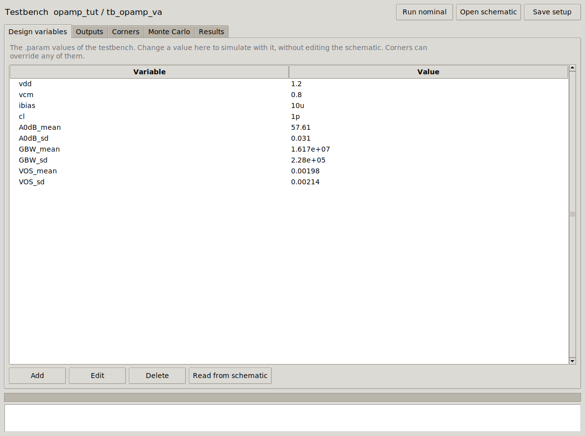
tb_opamp_vaand press Sim. Environment. - Tab Design variables: double-click each of the six
_meanand_sdvariables and type the values of the table. (vdd,vcm,ibias,clstay.) - Tab Monte Carlo: Number of runs 200, Starting run 1. The analysis variation only changes IHP’s transistor models, and this testbench has no transistors: leave it as it is.
- Run Monte Carlo.
4. Compare
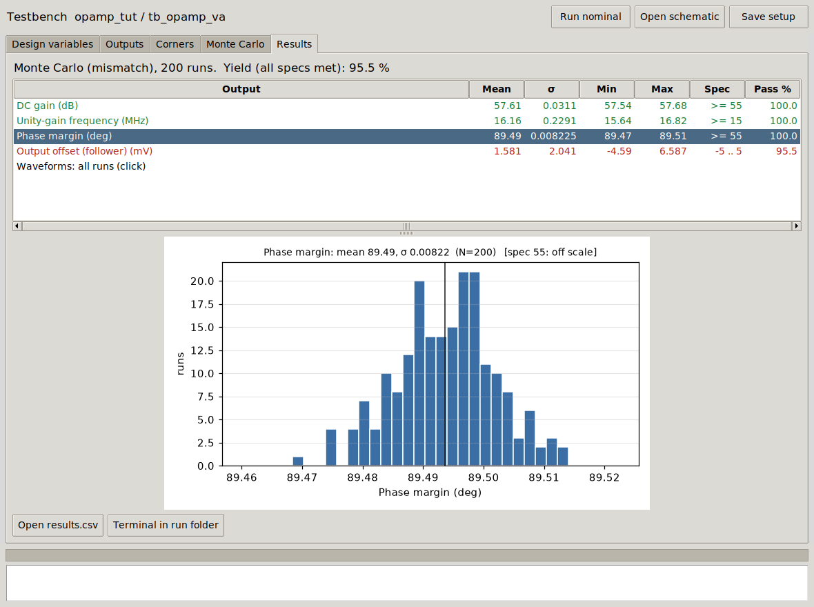
| Output (200 runs) | Transistors: mean ± σ | Model: mean ± σ |
|---|---|---|
| DC gain | 57.61 ± 0.031 dB | 57.61 ± 0.031 dB |
| Unity-gain frequency | 16.17 ± 0.228 MHz | 16.16 ± 0.229 MHz |
| Output offset | 1.72 ± 2.14 mV | 1.58 ± 2.04 mV |
| Offset yield (±5 mV) | 94.5 % | 95.5 % |
| Phase margin | 60.38 ± 0.30° | 89.49 ± 0.008° |
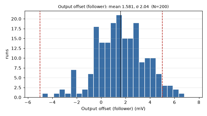
Gain, bandwidth and offset are reproduced: the differences (0.14 mV in the mean offset, 5 % in its σ) are what two independent sets of 200 samples give (the uncertainty of a mean is σ/√N = 2.14/√200 = 0.15 mV). The model’s Monte Carlo is as good as the transistors’ for everything the model contains.
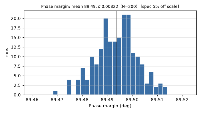
The phase margin is not reproduced at all: 89.5° in every run, while the transistors give 60.4° ± 0.3°. The model has no second pole, so it would say that any feedback circuit built with this op-amp is perfectly stable and never rings. That is the next step: your exercise.