
Chapter 5 of 14 · about 30 min
A behavioural model in Verilog-A
A behavioural model describes what the op-amp does with a few equations instead of eight transistors. It simulates much faster, and it is what you use when the op-amp is one block of a bigger system (a filter, an ADC). Here it will also let us run Monte Carlo without the transistors (chapter 10).
1. The model
Create the cell opamp_va with a Verilog-A view (File > New cell…, tick Verilog-A). It opens in the text editor. The model has the same pins as the transistor-level op-amp, so it can take its place in any testbench:
module opamp_va(INP, INN, OUT, IBIAS, VDD, VSS);
    inout INP, INN, OUT, IBIAS, VDD, VSS;
    electrical INP, INN, OUT, IBIAS, VDD, VSS;
    electrical n1;                      // internal node: the dominant pole

    parameter real A0dB    = 57.6;      // DC gain (dB)
    parameter real GBW     = 16.2e6;    // gain-bandwidth product (Hz)
    parameter real VOS     = 1.98e-3;   // input-referred offset (V)
    parameter real SR      = 10.6e6;    // slew rate (V/s)
    ...
    analog begin
        a0   = pow(10, A0dB / 20);
        gm   = 1e-3;                    // any value: only gm*r1 and gm/c1 matter
        r1   = a0 / gm;                 // DC gain a0 = gm * r1
        c1   = gm / (2 * `M_PI * GBW);  // unity gain at GBW
        imax = SR * c1;                 // slewing: c1 charged at most with imax
        vmid = (V(VDD) + V(VSS)) / 2;

        // input stage: limited transconductance into r1 // c1
        I(n1, VSS) <+ -imax * tanh(gm * (V(INP, INN) + VOS) / imax);
        I(n1, VSS) <+ (V(n1) - vmid) / r1;
        I(n1, VSS) <+ c1 * ddt(V(n1, VSS));

        // output: follows n1, kept VMARGIN away from the rails
        ...
        I(OUT, VSS) <+ (V(OUT) - vt) / ROUT;
    end
endmodule
The whole file, with comments, is in the reference library (opamp_tut/opamp_va/opamp_va.va). One pole (r1 and c1), slew-rate limiting (the tanh), output limits and supply current: four numbers taken from the transistor-level simulation describe the op-amp.
2. Compile it
Right-click opamp_va > Run > Compile Verilog-A (OpenVAF). OpenVAF writes opamp_va.osdi next to the source; the view Compiled model (OSDI) appears. Recompile after every change.
3. A symbol and a testbench
The model’s symbol is the same triangle, with a different netlist line: the instance is an OSDI device, N followed by its name, its pins and its model card. Copy opamp/opamp.sym to opamp_va/opamp_va.sym (in a terminal, or Terminal here on the view) and replace its K {...} block, in a text editor, by:
K {type=primitive
format="N@name @pinlist @model"
template="name=1 model=opamp_va_model"
}
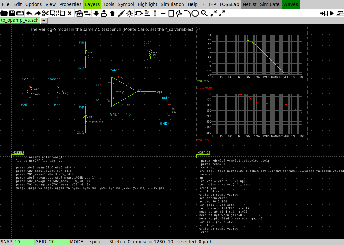
The pin order of the symbol (INP, INN, OUT, IBIAS, VDD, VSS) must be the module’s port order. The testbench tb_opamp_va is a copy of tb_opamp_ac with the model instead of the transistors. Its NGSPICE block loads the compiled model and defines the model card from design variables:
.param A0dB_mean=57.6 A0dB_sd=0
.param GBW_mean=16.2e6 GBW_sd=0
.param VOS_mean=1.98e-3 VOS_sd=0
.param A0dB_mc=agauss(A0dB_mean, A0dB_sd, 1)
.param GBW_mc=agauss(GBW_mean, GBW_sd, 1)
.param VOS_mc=agauss(VOS_mean, VOS_sd, 1)
.model opamp_va_model opamp_va A0dB={A0dB_mc} GBW={GBW_mc} VOS={VOS_mc} SR=10.6e6
.control
pre_osdi [file normalize [xschem get current_dirname]/../opamp_va/opamp_va.osdi]
...(pre_osdi loads the compiled model; the part in brackets is replaced by xschem with the absolute path of opamp_va.osdi when it writes the netlist. The agauss lines are for chapter 10: with the _sd variables at 0 they just give the mean values.)
4. Model versus transistors
| Transistors (tb_opamp_ac) | Verilog-A (tb_opamp_va) | |
|---|---|---|
| DC gain | 57.61 dB | 57.60 dB |
| Unity-gain frequency | 16.17 MHz | 16.20 MHz |
| Output offset | 1.73 mV | 1.71 mV |
| Phase margin | 60.4° | 89.5° |
Gain, bandwidth and offset agree. The phase margin does not: a one-pole model always has 90°. The real op-amp has a second pole at its output (from M6’s transconductance and the load) and the Miller zero. Keep this in mind: it is the subject of the exercise in chapter 11.
v(out) − v(inp). For the model this is VOS minus the gain error of a finite-gain follower, (VCM − VDD/2)/A0 = (0.8 − 0.6)/759 = 0.26 mV. So VOS = 1.73 + 0.26 ≈ 1.98 mV reproduces the transistor-level number.